Understanding Mechanistic Localization in detail- Rewiring LLMs
Mechanistic localization is a mechanistic interpretability approach where we try to identify where in a model’s computation a certain behavior happens. Instead of just saying “this neuron is correlated with X”, it asks “which exact weights, neurons, or circuits are responsible for producing X?”.
Think of it like reverse-engineering a neural network the same way you’d reverse-engineer a microchip: finding the parts of the circuit that actually implement a function.
Can it help determine why a model takes a decision?
✅ Yes, but with caveats:
-
It can pinpoint which internal components (layers, neurons, attention heads) are crucial for a given decision.
-
For example, in an LLM, mechanistic localization might identify that Attention Head 3.7 is carrying the subject–verb agreement signal that drives the output choice.
-
This helps explain why the model favored one prediction over another, but it’s at the mechanistic level of computation, not necessarily at the human-level reasoning you might expect.
Can it help identify which parameters impact output?
✅ Yes, partially:
-
By ablating (removing) or patching (replacing) specific neurons, attention heads, or weight matrices, you can measure how much the output changes.
-
This gives a causal estimate of which parameters are necessary for a given behavior.
-
Example: If zeroing out a subset of weights makes the model fail at sentiment classification, you’ve localized the “sentiment circuit”.
❌ Limits:
-
Large models have billions of parameters, and many decisions are highly distributed. You may find multiple redundant pathways.
-
Not every decision is “localized” to a neat, interpretable circuit — sometimes the knowledge is smeared across layers.
How it connects to your question
-
Why a model takes a decision → mechanistic localization can highlight which part of the computation is responsible.
-
Which parameters impact output → it can identify the causal subset of weights/neurons/heads that drive a behavior.
But: this is not the same as traditional feature importance (like SHAP or LIME). Instead of “feature X increased probability by 0.2”, mechanistic localization says:
“These 25 neurons and 3 attention heads in layer 12 are the circuit implementing the behavior.”
Mechanistic Localization vs. SHAP/LIME (Feature Attribution)
1. Level of Explanation
-
SHAP/LIME (Feature Attribution):
-
Works at the input–output level.
-
Tells you: “For this prediction, feature A contributed +0.3, feature B contributed –0.2.”
-
Great for tabular data or models with clear feature inputs.
-
Doesn’t explain how the model internally produced this.
-
-
Mechanistic Localization:
-
Works at the internal computation level.
-
Tells you: “Layer 7, Head 3.7 is carrying the subject–verb agreement signal, and these weights are essential for the output.”
-
Explains the circuitry inside the model, not just the input–output relationship.
-
2. Granularity
-
SHAP/LIME:
-
Feature importance → which input variables matter most.
-
Human-readable if inputs are understandable (age, salary, etc.).
-
-
Mechanistic Localization:
-
Neuron/weight/attention-head level → which exact parameters matter.
-
More technical, less human-friendly, but deeper causal insight.
-
3. Interpretability Goal
-
SHAP/LIME:
-
Goal: Transparency for end-users.
-
Useful in regulated industries (finance, healthcare) where you need to justify model predictions in simple terms.
-
-
Mechanistic Localization:
-
Goal: Scientific understanding of model internals.
-
Useful for AI safety, debugging, and steering model behavior (e.g., removing a bias circuit).
-
4. Causality vs Correlation
-
SHAP/LIME:
-
Attribution is often correlational.
-
Example: It might say “word X had high weight in prediction” but that doesn’t prove the model would fail if you remove the word.
-
-
Mechanistic Localization:
-
Uses interventions (ablations, patching).
-
Example: Knock out a neuron → if the model breaks, you know it’s causally involved.
-
5. When to Use Each
-
SHAP/LIME → When you want:
-
A human-readable explanation of why a prediction was made
-
Regulatory compliance (credit scoring, fraud detection)
-
Quick debugging of input sensitivity
-
-
Mechanistic Localization → When you want:
-
To reverse-engineer model circuits
-
To audit model safety (bias, memorization, failure modes)
-
To identify which parameters or subnetworks control a behavior
-
✅ Quick Analogy:
-
SHAP/LIME = Looking at a car dashboard to see which knobs (inputs) affect speed.
-
Mechanistic Localization = Opening the engine and tracing the wiring/gears that make the car move.
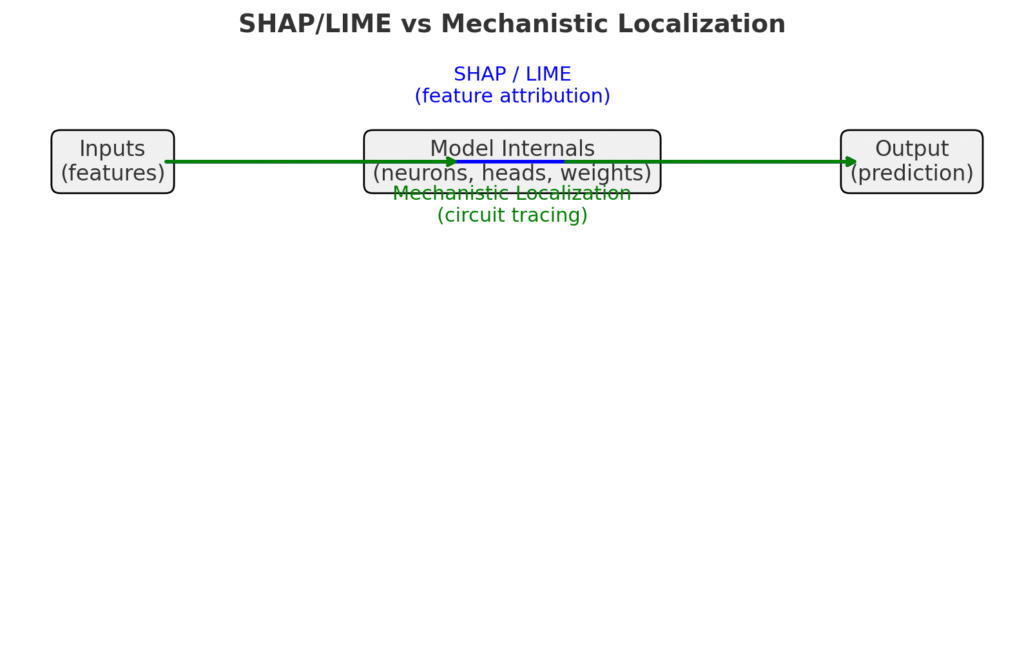
SHAP/LIME vs. Mechanistic Localization
| Aspect | SHAP / LIME (Feature Attribution) | Mechanistic Localization (Mechanistic Interpretability) |
|---|---|---|
| Level of Explanation | Input–output (features ↔ prediction) | Internal computation (neurons, heads, weights ↔ behavior) |
| Focus | Which input features contributed most | Which internal parameters/circuits implement the behavior |
| Granularity | Human-readable features (e.g., age, income, words) | Neurons, attention heads, subnetworks, weight matrices |
| Method | Perturbation of inputs, surrogate models | Ablations, patching, circuit tracing, causal interventions |
| Type of Insight | Correlational (feature importance) | Causal (removing part of circuit changes behavior) |
| Use Case | Model transparency, compliance, explaining decisions to end-users | Reverse-engineering, AI safety, debugging, editing or steering models |
| Interpretability Goal | Trust & usability for humans | Scientific/mechanistic understanding of networks |
| Analogy | Looking at a car dashboard to see which knobs affect speed | Opening the engine to see which gears/wires produce motion |
-
Blue (Top Path) = SHAP/LIME → Goes directly from Inputs → Outputs, showing which features influenced the prediction.
-
Green (Bottom Path) = Mechanistic Localization → Goes through the Model Internals, showing which neurons/weights drive the behavior.
Example: Sentiment Analysis on the sentence
👉 “The movie was surprisingly good, despite slow pacing.”
🔵 SHAP / LIME (Feature Attribution)
-
Works at input → output level.
-
Explanation:
-
Word “good” contributed +0.6 toward Positive.
-
Word “surprisingly” contributed +0.3 toward Positive.
-
Word “slow” contributed –0.4 toward Negative.
-
Overall → classified as Positive.
-
-
Takeaway: You see which words (features) mattered most for the decision.
🟢 Mechanistic Localization (Inside Model Circuits)
-
Works at internal computation level.
-
Explanation:
-
Identified that Attention Head 5.3 tracks positive sentiment words.
-
Neuron cluster in Layer 12 amplifies “surprisingly good” and suppresses “slow pacing”.
-
Ablation: if we remove Head 5.3, the model stops correctly identifying “good” as positive.
-
-
Takeaway: You see which neurons/heads/weights caused the decision inside the model.
✅ Side-by-Side Summary
| Method | What it Tells You | Example Here |
|---|---|---|
| SHAP / LIME | Feature-level contribution | Words “good” (+0.6), “slow” (–0.4), “surprisingly” (+0.3) drove the output |
| Mechanistic Localization | Circuit-level explanation | Attention Head 5.3 + Neurons in Layer 12 implement the “positive sentiment” pathway |
🔑 Big Picture:
-
SHAP/LIME → User-friendly, tells which words influenced the result.
Example: Loan Approval Model
👉 Input:
-
Age: 28
-
Income: ₹70,000/month
-
Credit Score: 720
-
Existing Loans: 1
-
Employment: Full-time
Model Output: ✅ Approved
🔵 SHAP / LIME (Feature Attribution)
-
Looks at inputs → output.
-
Explanation:
-
Credit Score 720 contributed +0.5 toward approval.
-
Stable Full-time Employment contributed +0.3.
-
Existing Loan contributed –0.2 (risk factor).
-
Income ₹70,000 contributed +0.2.
-
-
Takeaway: You know which applicant features drove approval, in numbers easy to show regulators or customers.
🟢 Mechanistic Localization (Inside Model Circuits)
-
Looks at internal network parameters → output.
-
Explanation:
-
Hidden Neuron Cluster in Layer 3 encodes “financial stability signal” (combining income + employment).
-
Neuron Pathway in Layer 5 strongly activates for high credit scores.
-
If we ablate (remove) the “credit score pathway neurons”, the model fails to distinguish 720 vs 600 scores.
-
If we patch in neurons from a rejected case (e.g., low credit score), approval flips to ❌ Rejected.
-
-
Takeaway: We’ve localized the internal circuits that implement “creditworthiness”.
✅ Side-by-Side Summary
| Method | What it Tells You | Example Here |
|---|---|---|
| SHAP / LIME | Which features mattered most | Credit score (+0.5), Employment (+0.3), Income (+0.2), Existing loan (–0.2) |
| Mechanistic Localization | Which neurons/weights implement the logic | Layer 3 encodes stability, Layer 5 encodes credit score → these circuits caused approval |
🔑 Big Picture:
-
SHAP/LIME = “Loan approved because credit score & income outweighed existing loan.”
-
Mechanistic Localization = “These neurons/layers implement the ‘credit score + income’ approval pathway.”
Source – https://arxiv.org/html/2410.12949v2